Enhancing Energy Management: Advanced Techniques for Forecasting and Optimization
Enhancing Energy Management: Advanced Techniques for Forecasting and Optimization
Mahim Rahaman, REU Scholar (Lehman college)
Under the guidance of Dr. Zhen Ni
NSF REU IN SENSING AND SMART SYSTEMS – FAU 2024
Infrastructure Systems: Machine Learning Techniques for Energy Forecasting and Optimization
Background
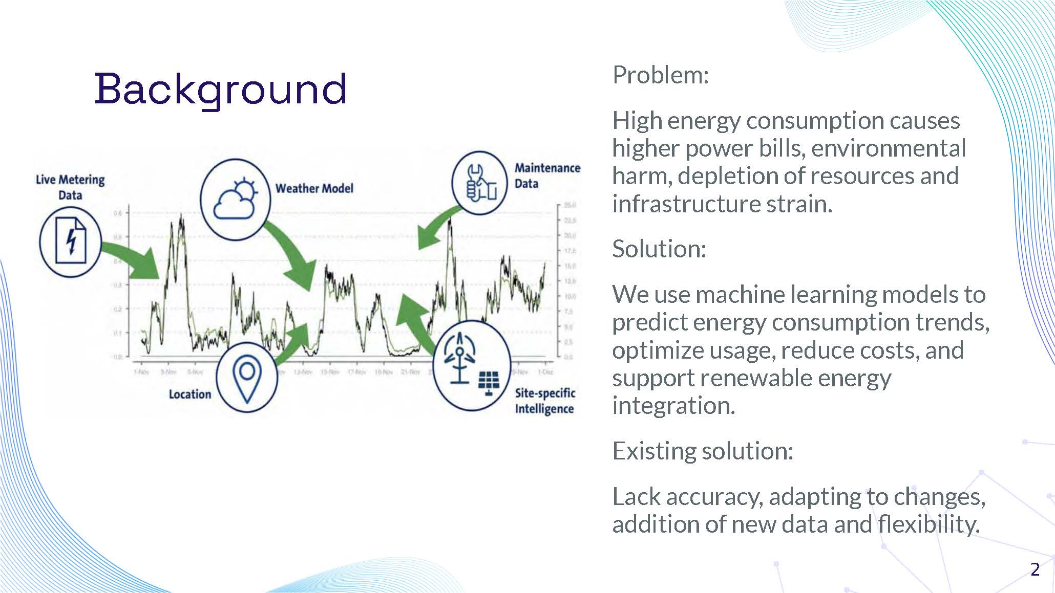
Problem:
High energy consumption causes higher power bills, environmental harm, depletion of resources and infrastructure strain.
Solution:
We use machine learning models to predict energy consumption trends, optimize usage, reduce costs, and support renewable energy integration.
Existing solution:
Lack accuracy, adapting to changes, addition of new data and flexibility.
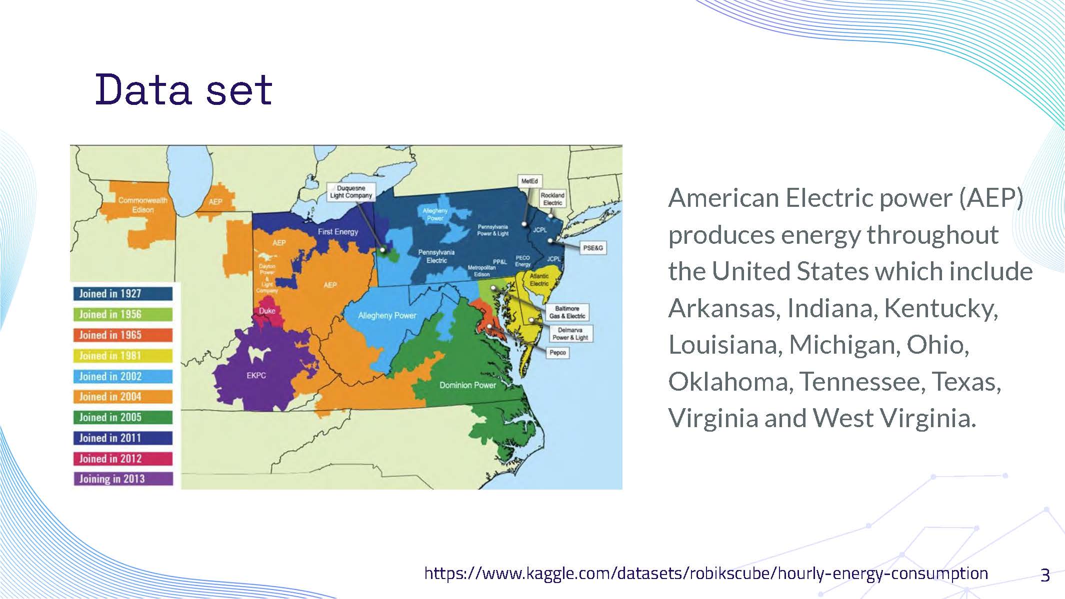
Data set information about American Electric Power (AEP) covering multiple US states
American Electric power (AEP) produces energy throughout the United States which include Arkansas, Indiana, Kentucky, Louisiana, Michigan, Ohio, Oklahoma, Tennessee, Texas, Virginia and West Virginia.
https://www.kaggle.com/datasets/robikscube/hourly-energy-consumption
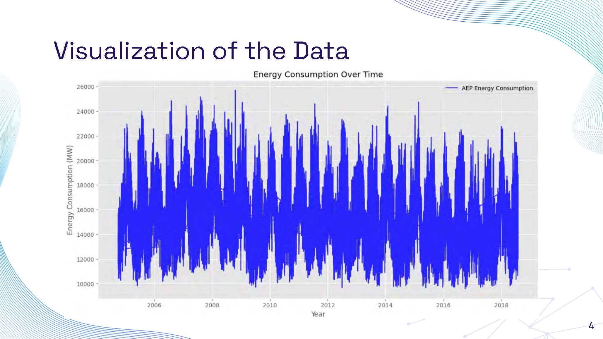
Visualization of the Data showing time series energy consumption
This slide contains a time series line graph showing energy consumption patterns over time. The graph displays hourly energy consumption data with fluctuations showing daily, weekly, and seasonal patterns in energy usage. The y-axis represents energy consumption in megawatts (MW) and the x-axis represents time periods. The visualization shows varying consumption levels with peaks and valleys indicating different usage patterns throughout the time series.
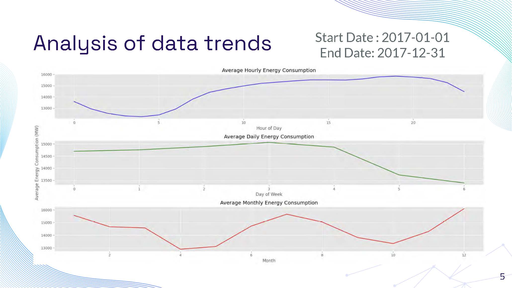
Analysis of data trends
Start Date : 2017-01-01
End Date: 2017-12-31
This slide contains a detailed time series visualization showing energy consumption trends throughout 2017. The graph displays seasonal variations with higher consumption during summer and winter months, and lower consumption during spring and fall. Daily patterns show regular fluctuations with peak usage during daytime hours and reduced consumption at night. Weekly patterns indicate differences between weekday and weekend consumption levels.
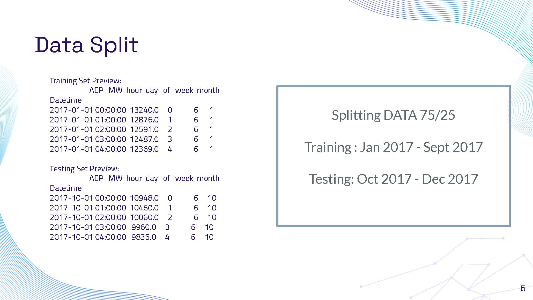
Data Split
Splitting DATA 75/25
Training : Jan 2017 - Sept 2017
Testing: Oct 2017 - Dec 2017
Training Set Preview:
| Datetime | AEP_MW | hour | day_of_week | month |
|---|---|---|---|---|
| 2017-01-01 00:00:00 | 13240.0 | 0 | 6 | 1 |
| 2017-01-01 01:00:00 | 12876.0 | 1 | 6 | 1 |
| 2017-01-01 02:00:00 | 12591.0 | 2 | 6 | 1 |
| 2017-01-01 03:00:00 | 12487.0 | 3 | 6 | 1 |
| 2017-01-01 04:00:00 | 12369.0 | 4 | 6 | 1 |
Testing Set Preview:
| Datetime | AEP_MW | hour | day_of_week | month |
|---|---|---|---|---|
| 2017-10-01 00:00:00 | 10948.0 | 0 | 6 | 10 |
| 2017-10-01 01:00:00 | 10460.0 | 1 | 6 | 10 |
| 2017-10-01 02:00:00 | 10060.0 | 2 | 6 | 10 |
| 2017-10-01 03:00:00 | 9960.0 | 3 | 6 | 10 |
| 2017-10-01 04:00:00 | 9835.0 | 4 | 6 | 10 |
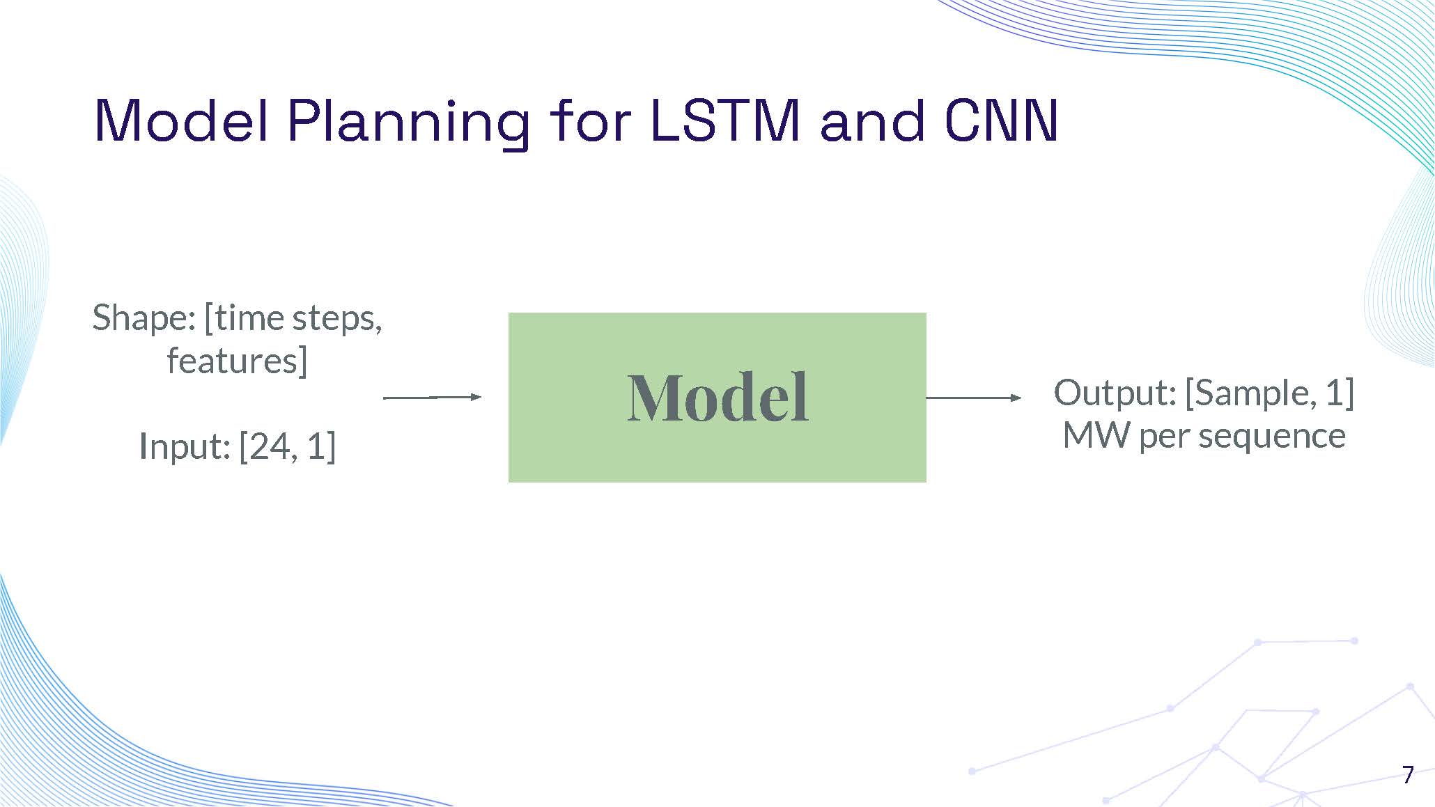
Model Planning for LSTM and CNN
Model
Shape: [time steps, features]
Input: [24, 1]
Output: [Sample, 1]
MW per sequence
This slide contains a diagram showing the model architecture planning. The diagram illustrates the input shape of [24, 1] representing 24 time steps with 1 feature, flowing through the model to produce an output shape of [Sample, 1] representing MW per sequence. The visualization shows the data flow and transformation through the neural network architecture.
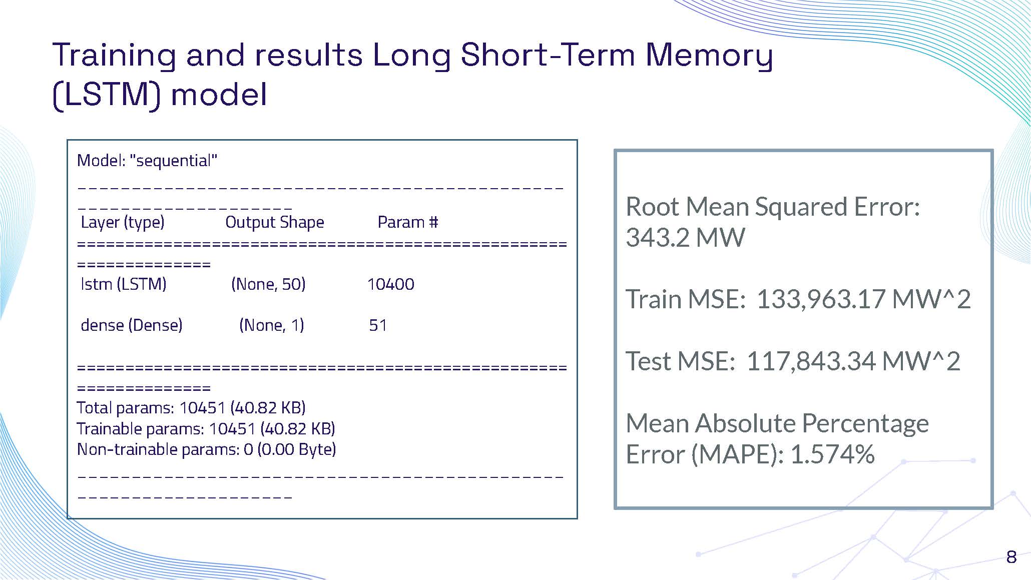
Training and results Long Short-Term Memory (LSTM) model
Root Mean Squared Error: 343.2 MW
Train MSE: 133,963.17 MW^2
Test MSE: 117,843.34 MW^2
Mean Absolute Percentage Error (MAPE): 1.574%
Model: "sequential"
_________________________________________________________________
| Layer (type) | Output Shape | Param # |
|---|---|---|
| lstm (LSTM) | (None, 50) | 10400 |
| dense (Dense) | (None, 1) | 51 |
=================================================================
Total params: 10451 (40.82 KB)
Trainable params: 10451 (40.82 KB)
Non-trainable params: 0 (0.00 Byte)
_________________________________________________________________
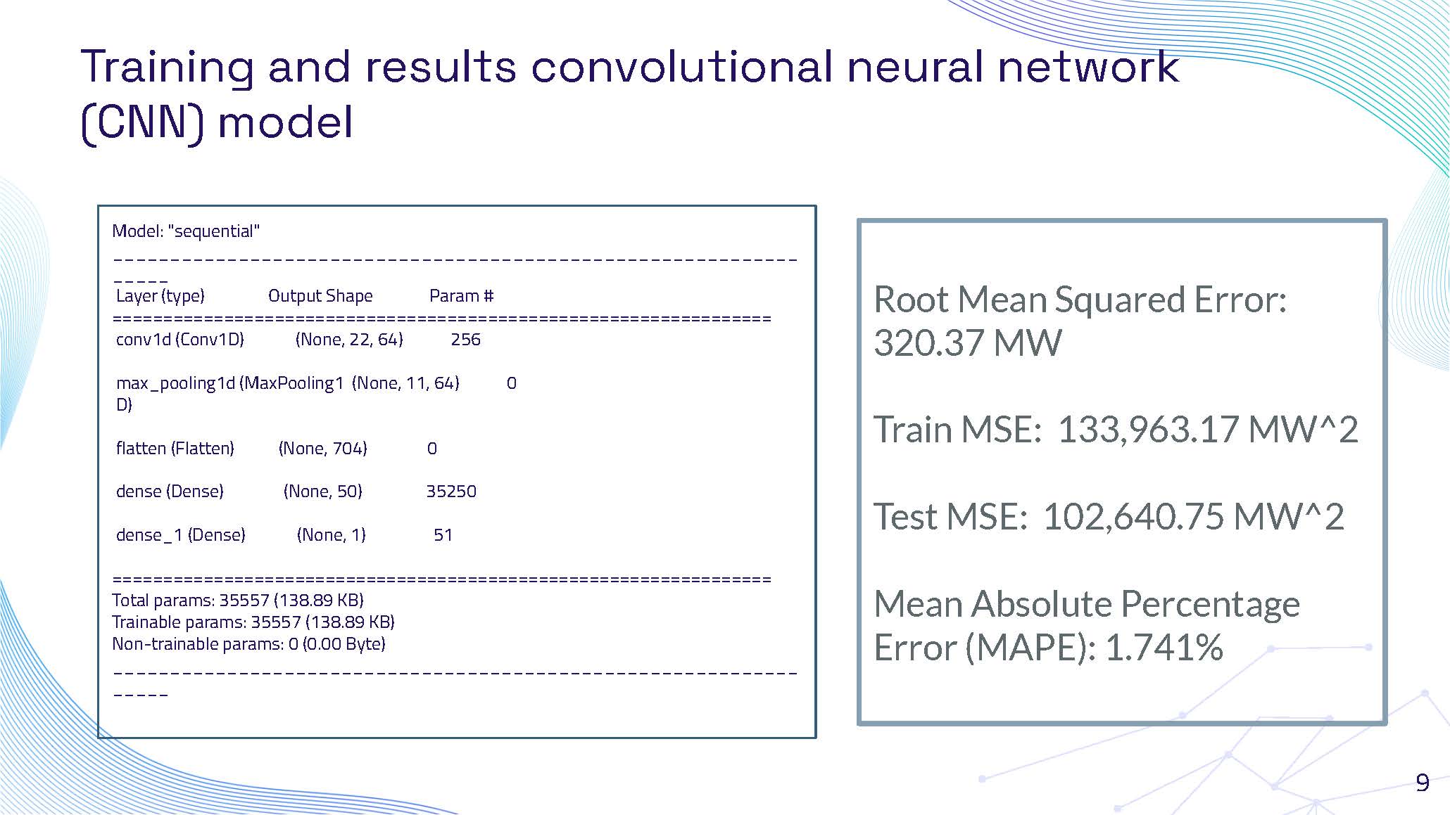
Training and results convolutional neural network (CNN) model
Model: "sequential"
=================================================================
| Layer (type) | Output Shape | Param # |
|---|---|---|
| conv1d (Conv1D) | (None, 22, 64) | 256 |
| max_pooling1d (MaxPooling1D) | (None, 11, 64) | 0 |
| flatten (Flatten) | (None, 704) | 0 |
| dense (Dense) | (None, 50) | 35250 |
| dense_1 (Dense) | (None, 1) | 51 |
=================================================================
Total params: 35557 (138.89 KB)
Trainable params: 35557 (138.89 KB)
Non-trainable params: 0 (0.00 Byte)
=================================================================
Root Mean Squared Error: 320.37 MW
Train MSE: 133,963.17 MW^2
Test MSE: 102,640.75 MW^2
Mean Absolute Percentage Error (MAPE): 1.741%
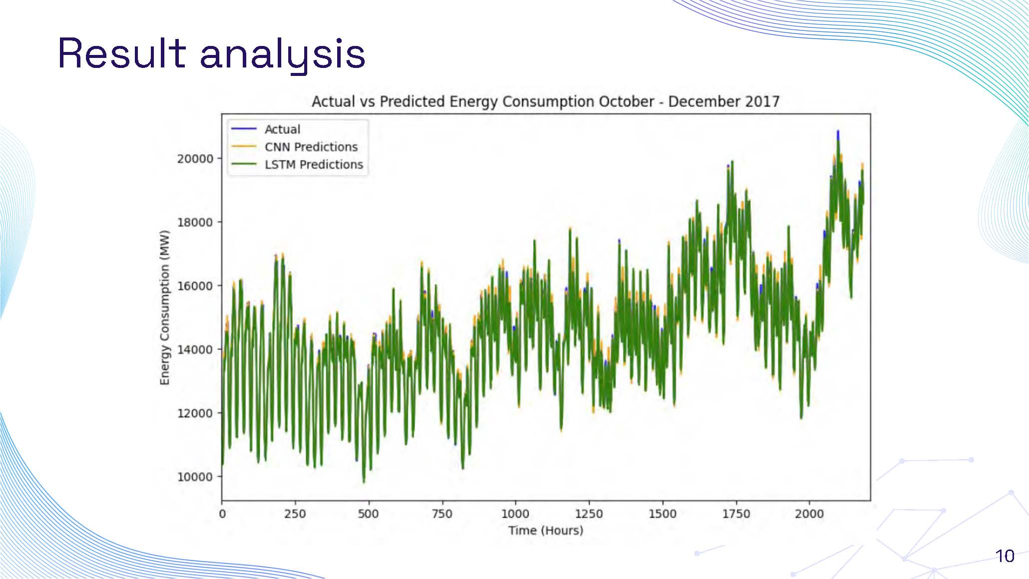
Result analysis showing comparative performance visualization
This slide contains a comparative visualization showing the performance analysis of different models. The graph displays predicted versus actual energy consumption values, allowing for visual comparison of model accuracy. The visualization shows how well each model captures the patterns in the energy consumption data, with lines representing different model predictions against the actual consumption values.
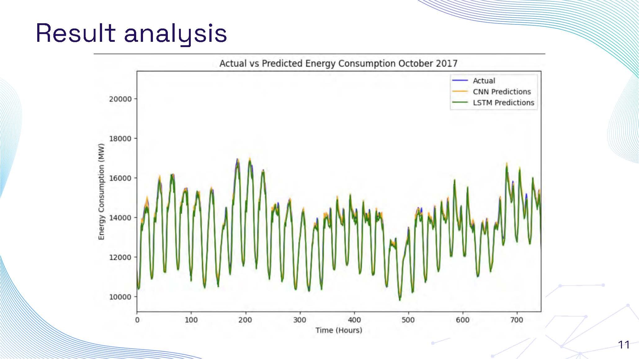
Result analysis continuation with additional performance metrics visualization
This slide continues the result analysis with additional performance visualization. The graph shows detailed comparison between predicted and actual values over time, highlighting the accuracy of different model predictions. The visualization demonstrates the models' ability to capture both short-term fluctuations and longer-term trends in energy consumption patterns.
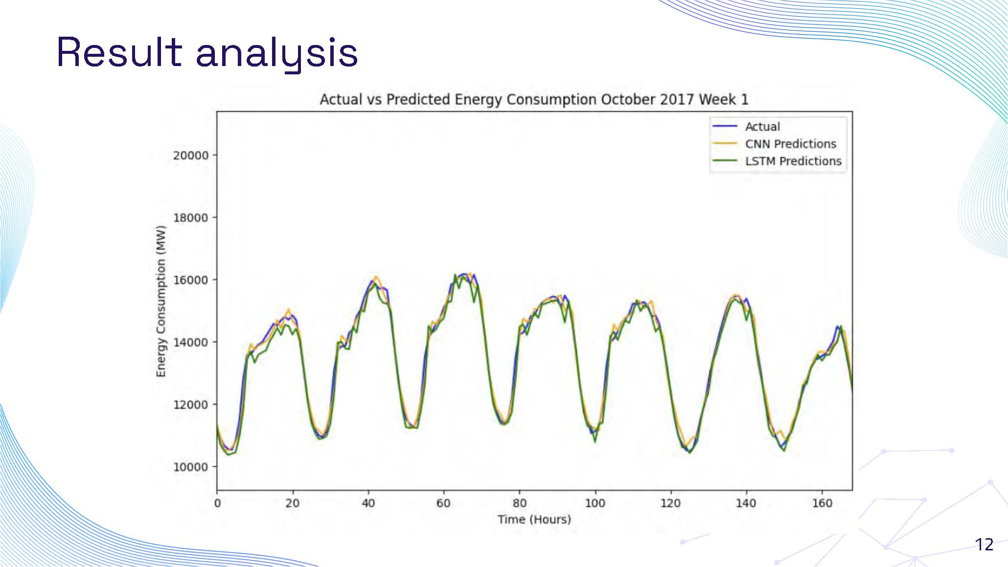
Result analysis final comparison showing model performance across different time periods
This slide presents the final result analysis with comprehensive model performance comparison. The visualization shows how different models perform across various time periods and conditions, highlighting their strengths and weaknesses in predicting energy consumption. The graph demonstrates the models' effectiveness in capturing seasonal variations, daily patterns, and unexpected fluctuations in energy demand.
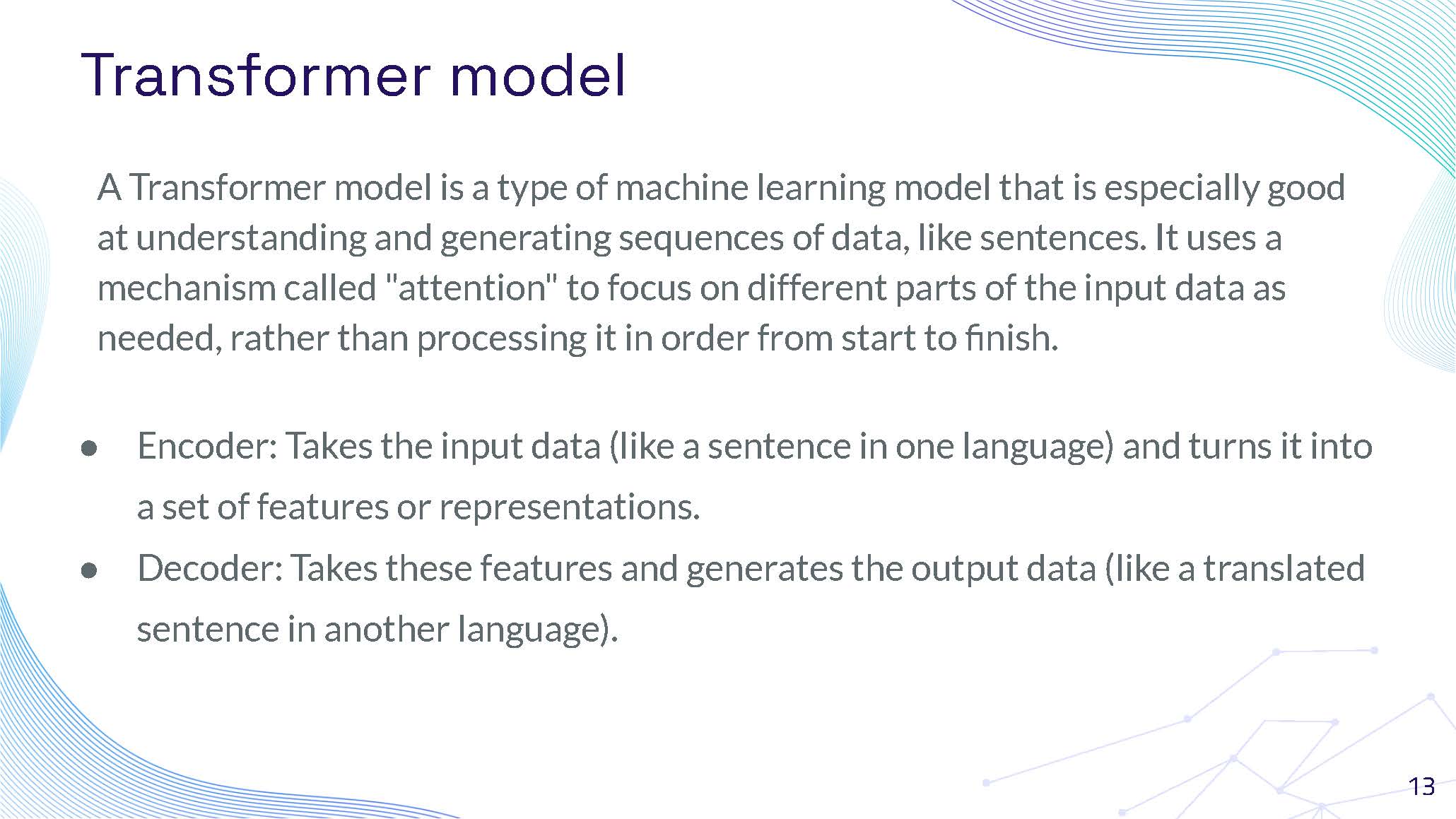
Transformer model explanation with encoder-decoder architecture description
A Transformer model is a type of machine learning model that is especially good at understanding and generating sequences of data, like sentences. It uses a mechanism called "attention" to focus on different parts of the input data as needed, rather than processing it in order from start to finish.
● Encoder: Takes the input data (like a sentence in one language) and turns it into a set of features or representations.
● Decoder: Takes these features and generates the output data (like a translated sentence in another language).
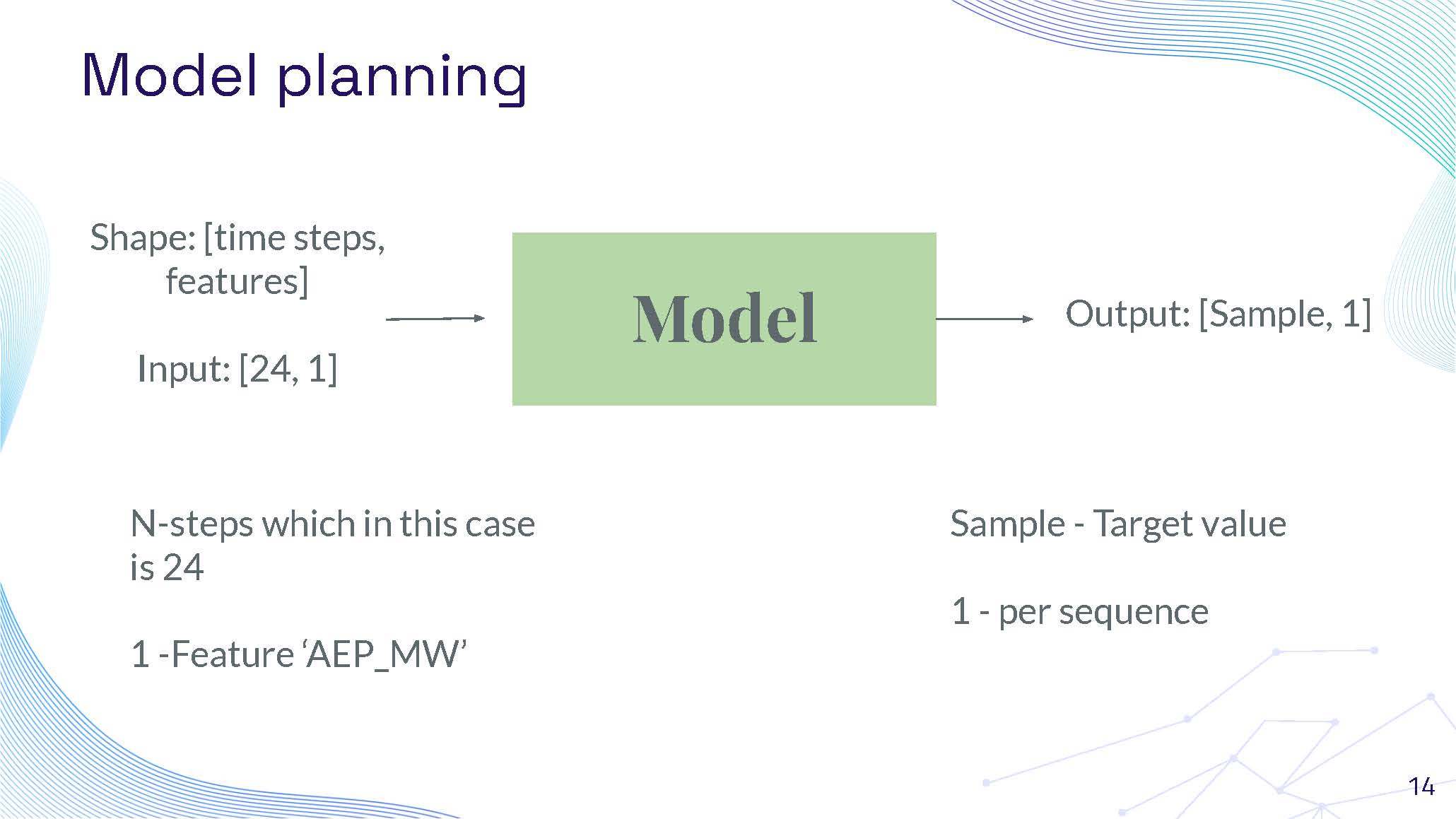
Model planning for Transformer showing input/output specifications
Model
Shape: [time steps, features]
Input: [24, 1]
Output: [Sample, 1]
N-steps which in this case is 24
1 -Feature 'AEP_MW'
Sample - Target value
1 - per sequence
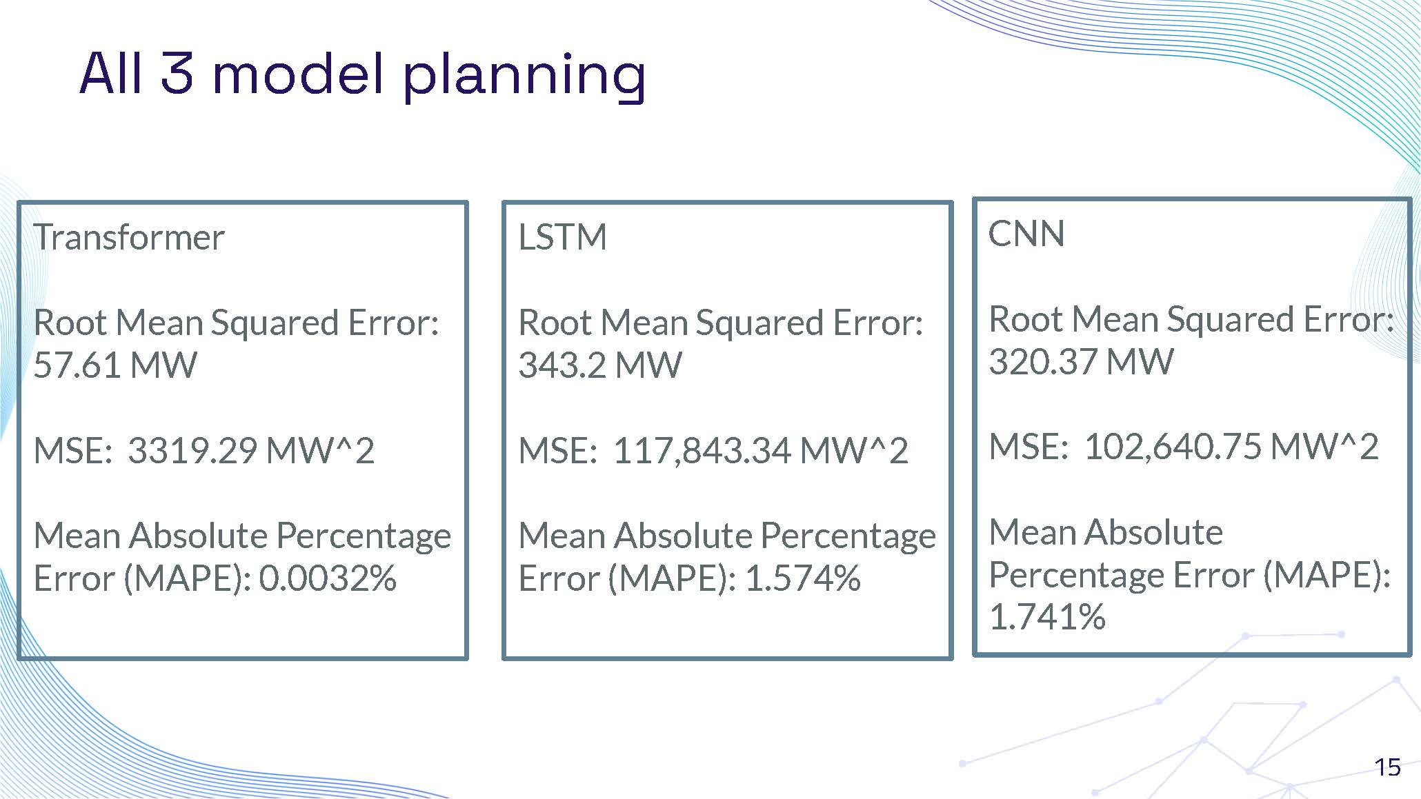
All 3 model planning results
Transformer
Root Mean Squared Error: 57.61 MW
MSE: 3319.29 MW^2
Mean Absolute Percentage Error (MAPE): 0.0032%
LSTM
Root Mean Squared Error: 343.2 MW
MSE: 117,843.34 MW^2
Mean Absolute Percentage Error (MAPE): 1.574%
CNN
Root Mean Squared Error: 320.37 MW
MSE: 102,640.75 MW^2
Mean Absolute Percentage Error (MAPE): 1.741%
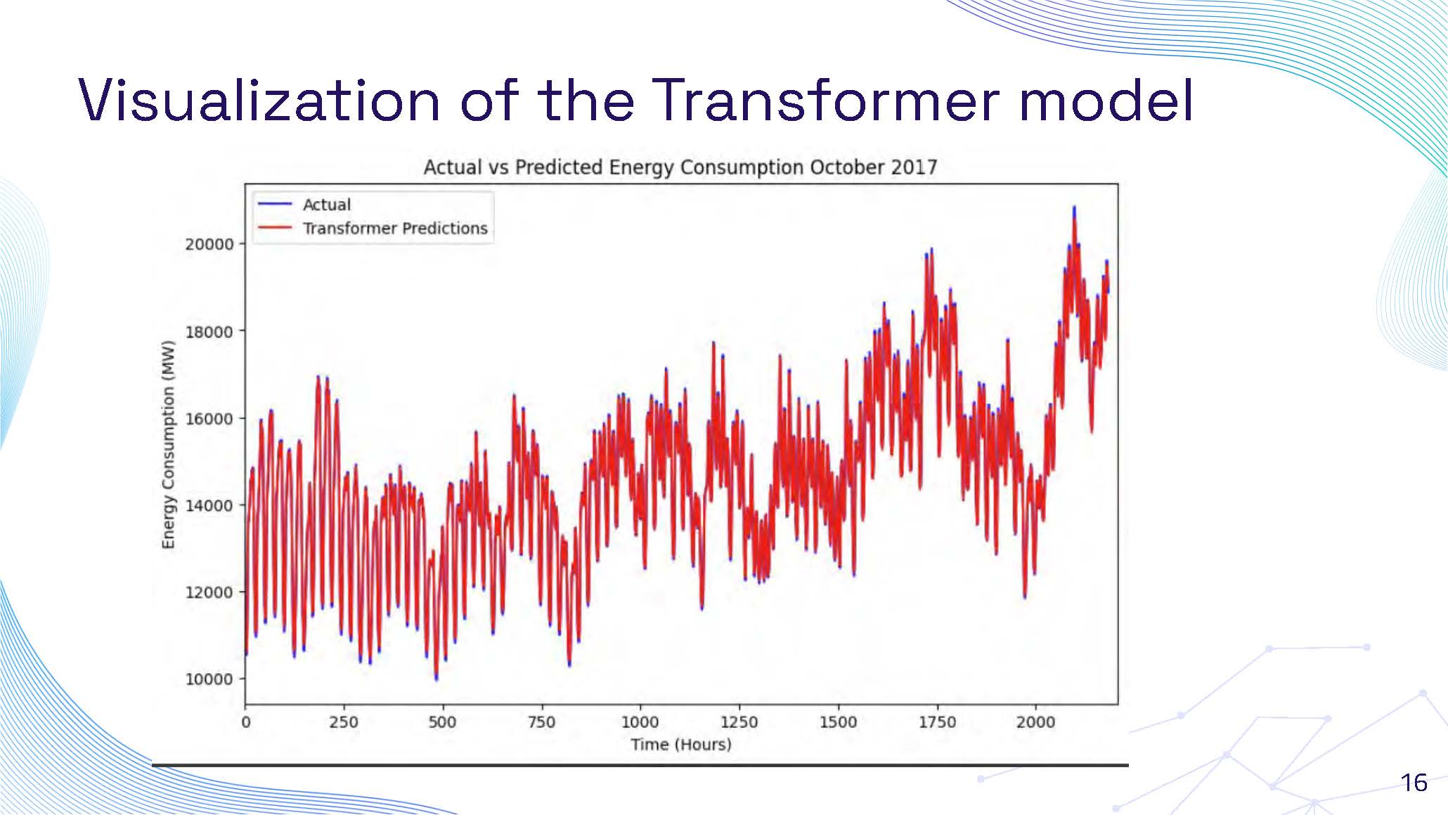
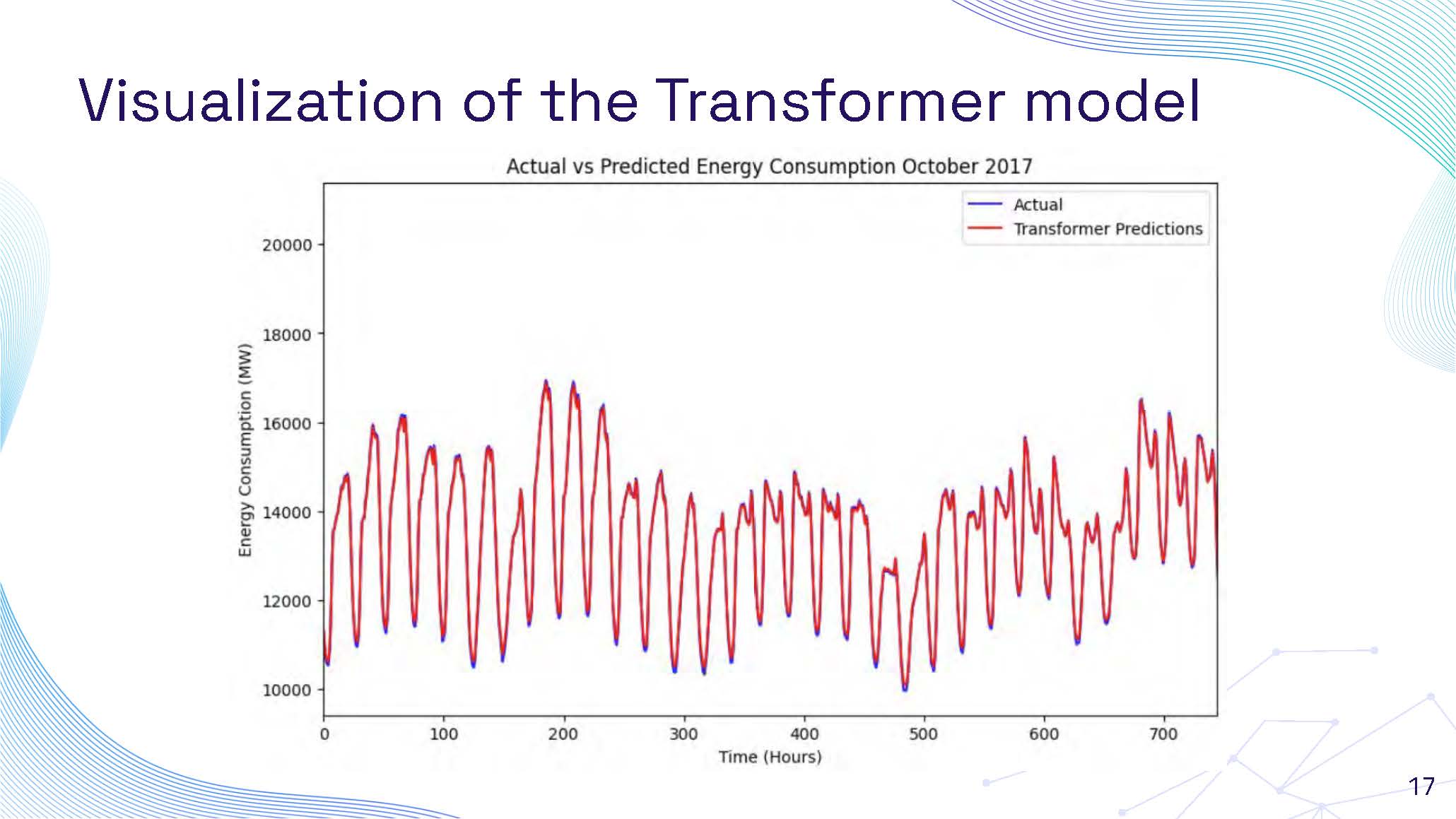
Visualization of the Transformer model showing predicted vs actual values
This slide displays a detailed visualization of the Transformer model's performance. The graph shows the comparison between predicted and actual energy consumption values, demonstrating the model's exceptional accuracy. The visualization reveals how closely the Transformer model predictions align with the actual consumption patterns, showing minimal deviation and excellent capture of both trends and variations in the energy data.
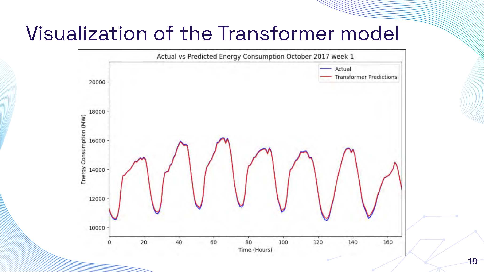
Visualization of the Transformer model showing detailed performance analysis
This slide continues the Transformer model visualization with additional detailed analysis. The graph presents a closer examination of the model's predictive capabilities, showing how the Transformer captures fine-grained patterns in energy consumption. The visualization demonstrates the model's superior performance in handling complex temporal dependencies and its ability to make accurate short-term and long-term predictions.
Visualization of the Transformer model showing comprehensive performance metrics
This slide presents the final comprehensive visualization of the Transformer model's performance. The graph shows the complete analysis of the model's predictive accuracy across different time periods and conditions. The visualization highlights the Transformer's exceptional ability to maintain high accuracy throughout various scenarios, demonstrating consistent performance and reliability in energy consumption forecasting.
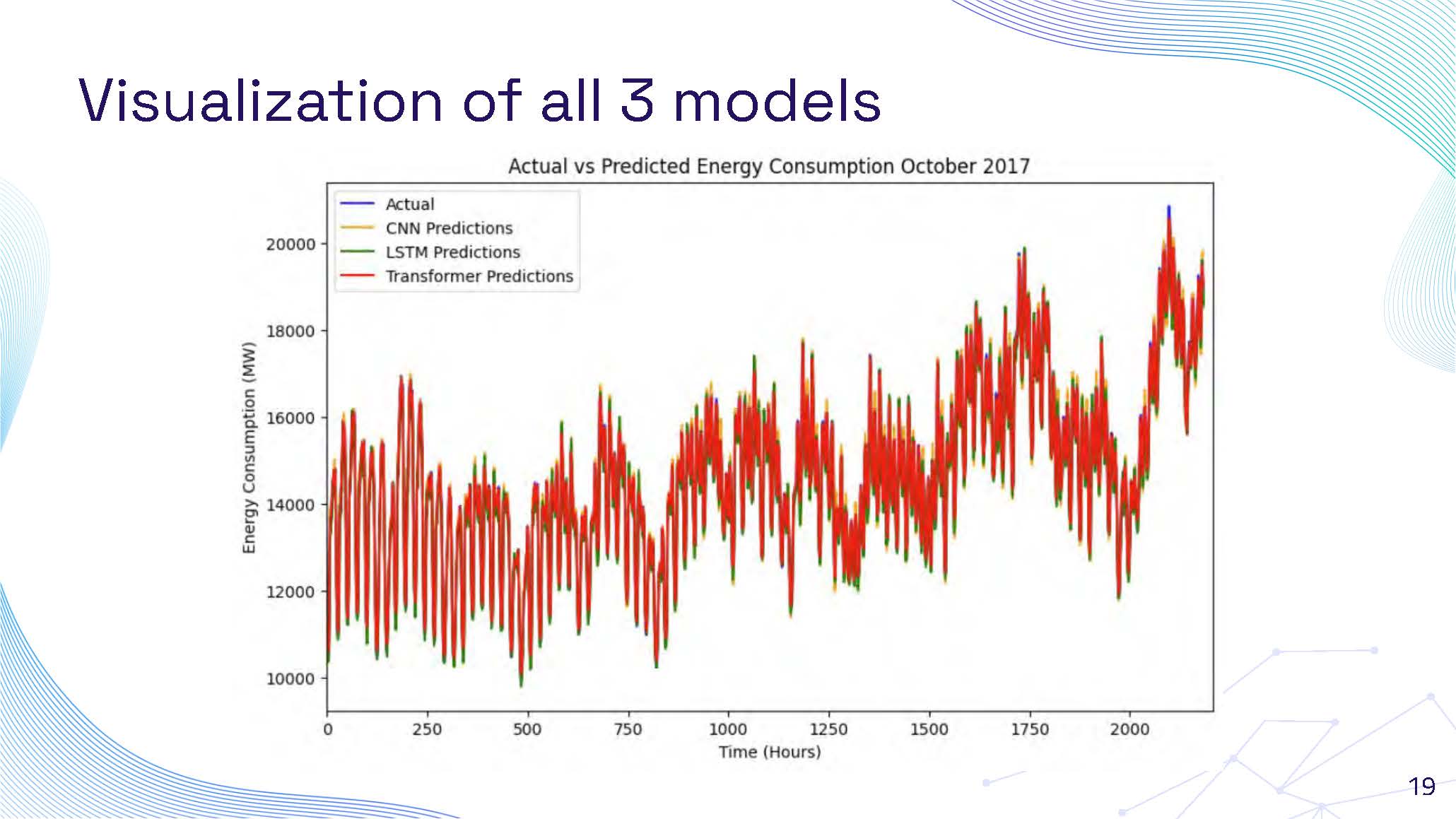
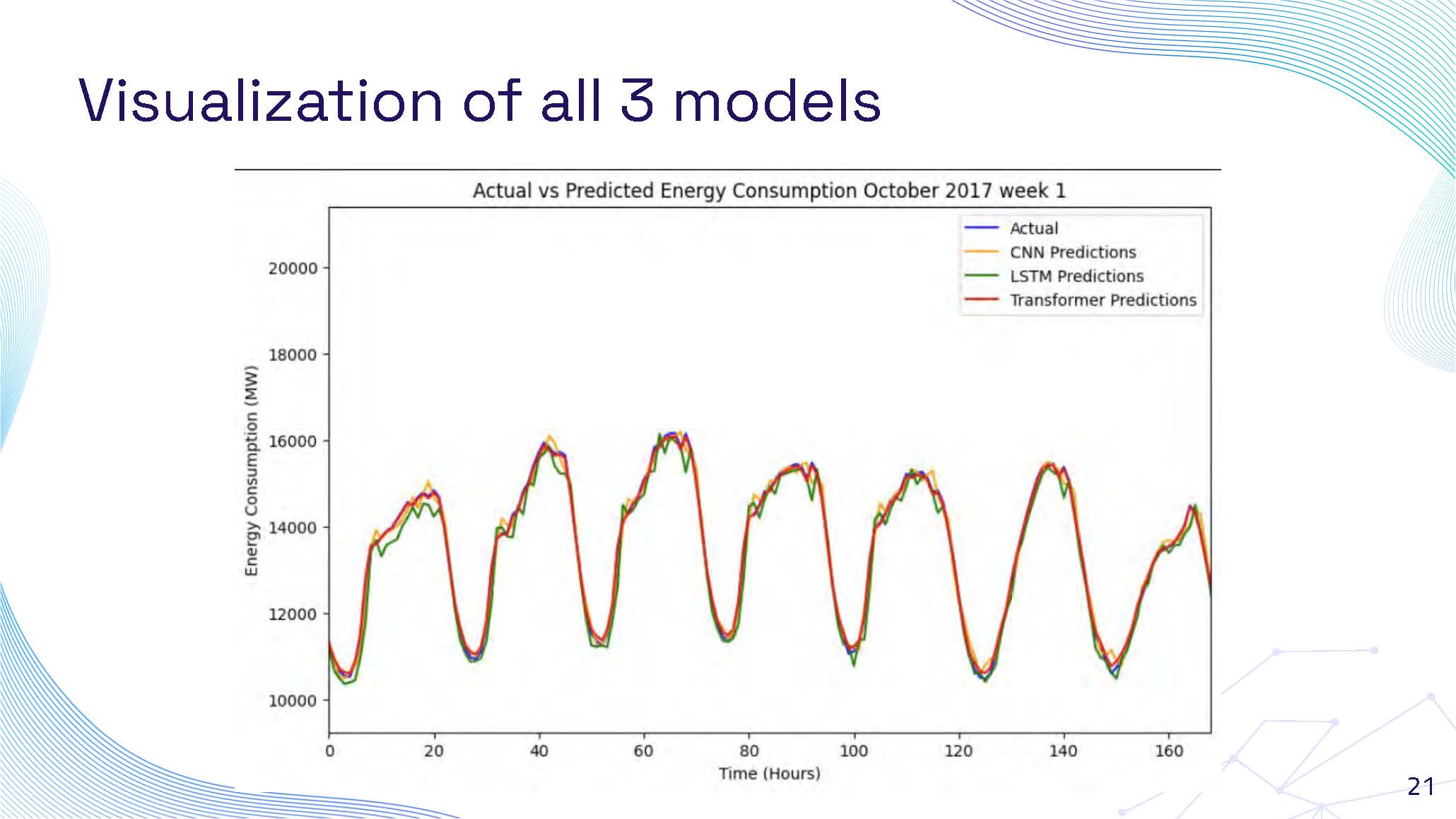
Visualization of all 3 models showing performance differences
This slide presents a comparative visualization of all three models (Transformer, LSTM, and CNN) performance. The graph shows side-by-side comparison of predicted versus actual energy consumption values for each model. The visualization clearly demonstrates the superior performance of the Transformer model with its closer alignment to actual values, while also showing the performance characteristics of LSTM and CNN models. This comparison highlights the differences in accuracy and prediction quality across the three different machine learning approaches.
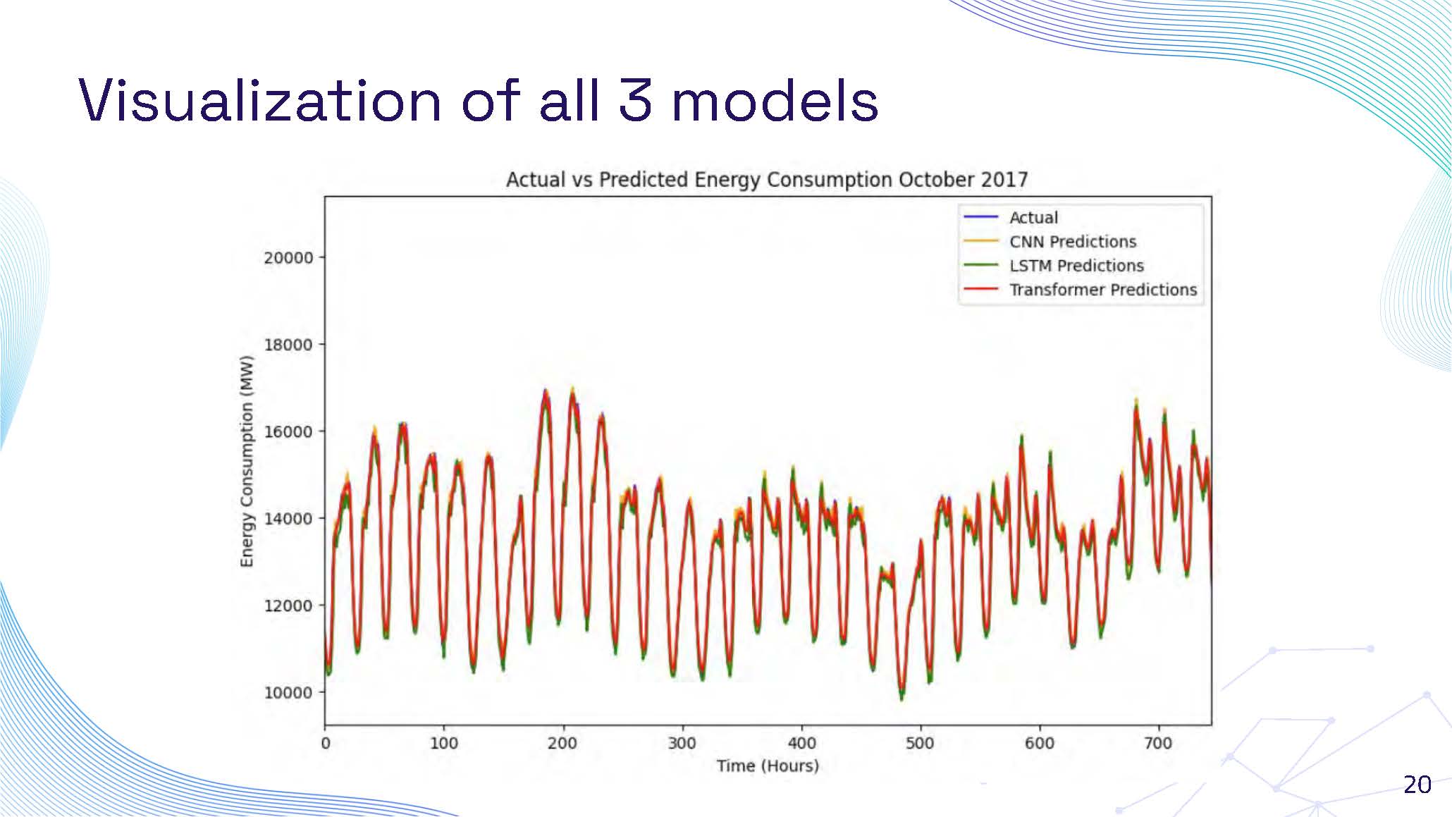
Visualization of all 3 models with detailed analysis
This slide continues the comparative analysis of all three models with detailed visualization. The graph provides an in-depth comparison showing how each model handles different aspects of energy consumption prediction. The visualization reveals the strengths and limitations of each approach, with the Transformer model showing superior accuracy, while LSTM and CNN models demonstrate their respective capabilities and areas where they perform well or face challenges in prediction accuracy.
Visualization of all 3 models summarizing performance results
This slide presents the final comparative visualization summarizing the performance of all three models. The comprehensive graph shows the complete analysis of Transformer, LSTM, and CNN models across various metrics and time periods. The visualization provides a conclusive comparison demonstrating the Transformer model's outstanding performance with significantly lower error rates, while also acknowledging the contributions and specific use cases where LSTM and CNN models may still provide value in energy consumption forecasting applications.
Conclusion
Transformer models ability to use:
● Attention Mechanism
● Parallel processing
● Scalability
● Flexibility
● Long-range Dependencies

Future improvements
Future implementation of new and challenging dataset will make this project more advanced and improve the way we consume our energy.
Reference
Bryant, M. (n.d.). Electric vehicle charging dataset [Data set]. Kaggle. Retrieved from https://www.kaggle.com/datasets/michaelbryantds/electric-vehicle-charging-dataset
Robikscube. (n.d.). Hourly energy consumption [Data set]. Kaggle. Retrieved from https://www.kaggle.com/datasets/robikscube/hourly-energy-consumption
Qingsong. (n.d.). Time-series transformers: A comprehensive review [GitHub repository]. GitHub. Retrieved from https://github.com/qingsongedu/time-series-transformers-review
Intel Tech. (2021, April 30). How to apply transformers to time-series models: Spacetimeformer. Medium. Retrieved from https://medium.com/intel-tech/how-to-apply-transformers-to-time-series-models-spacetimeformer-e452f2825d2e
Hugging Face. (n.d.). Time series transformer. Retrieved from https://huggingface.co/docs/transformers/en/model_doc/time_series_transformer

End of Presentation
Click the right arrow to return to the beginning of the slide show.
For a downloadable version of this presentation, email: I-SENSE@FAU.