Battery-Free Underwater Wireless Communication Sensors Using Scatter Communication Principles

Summer 2022 FAU iSENSE REU

Presented by Parker Wilmoth, Tariq Wardak, and Ynes Ineza

REU Mentor: Dr. Sklivanitis

Why We Need Underwater IoT

The Problem with Underwater Wireless Today

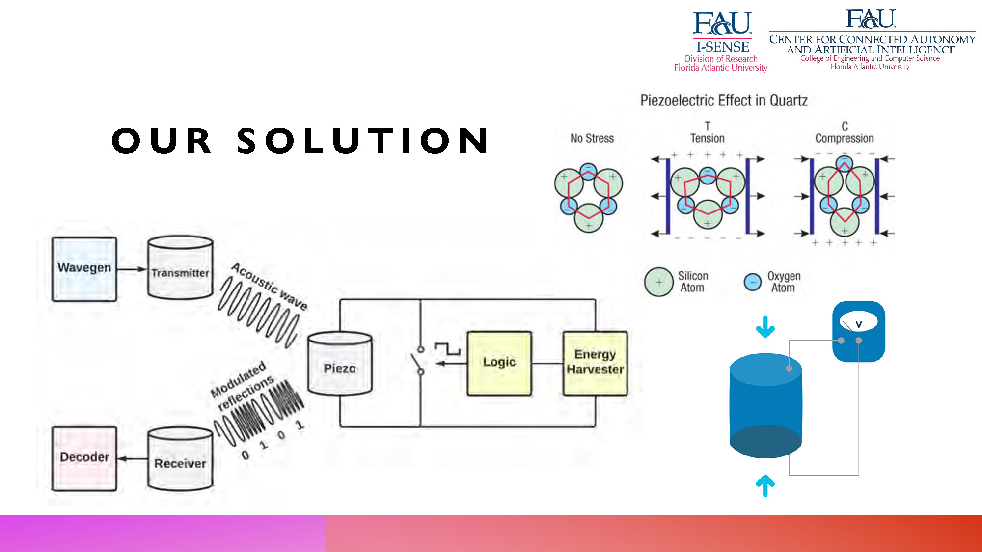
Our Solution

Diagrams showing:

• Wavegen, transmitter, acoustic wave, piezo, logic, energy harvester, receiver, and decoder.
• Piezoelectric effect in quartz under no stress, tension, and compression, with silicon and oxygen atoms labeled.
• A blue cylindrical component connected to a voltmeter symbol.

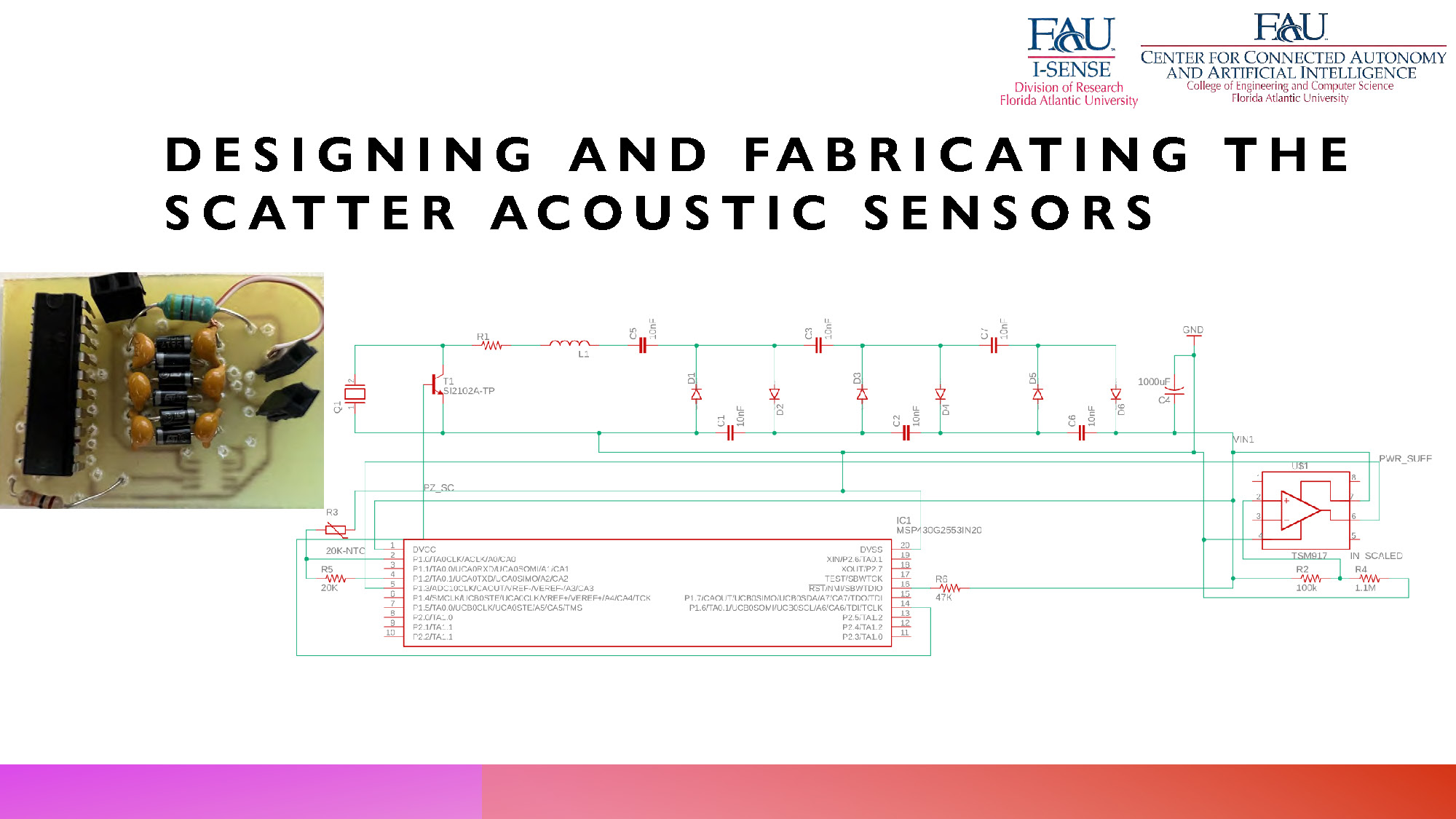
Designing and Fabricating the Scatter Acoustic Sensors

Elements shown:

• Photograph of an electronic circuit board with components.
• Electronic schematic diagram with labeled components including resistors, capacitors, diodes, transistors, microcontroller (MSP30G2553IN20), and operational amplifier (TSM917).

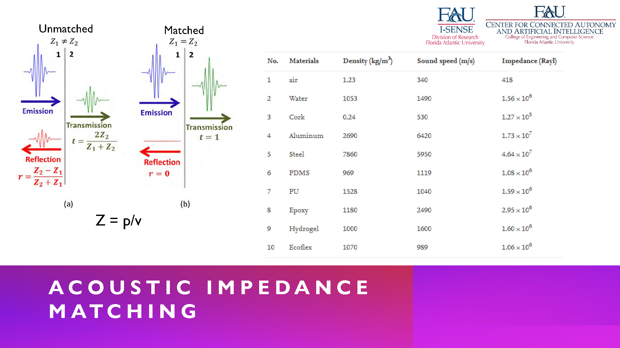
Acoustic Impedance Matching

The image displays two diagrams. The first diagram, labeled "(a) Unmatched," shows an "Emission" wave that reflects and transmits with the labels $r = \frac{Z_2 - Z_1}{Z_2 + Z_1}$ and $t = \frac{2Z_2}{Z_1 + Z_2}$. The second diagram, labeled "(b) Matched," shows an "Emission" wave with no reflection ($r=0$) and full transmission ($t=1$). Below the diagrams is the equation $Z = \rho v$. The top right has a table with four columns: "No.," "Materials," "Density (kg/m^3)," "Sound speed (m/s)," and "Impedance (Rayl)." The table has 10 rows of data for various materials, including air, water, cork, aluminum, steel, PDMS, PU, epoxy, hydrogel, and ecoflex.

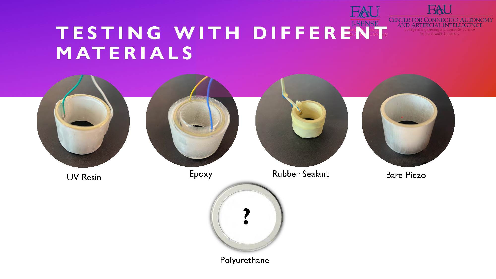
Testing with Different Materials

Below are five circular images showing a component, possibly a piezo, with wires attached. The first four are labeled "UV Resin," "Epoxy," "Rubber Sealant," and "Bare Piezo," respectively. The fifth image is labeled "Polyurethane" and has a question mark inside a white circle in the center.

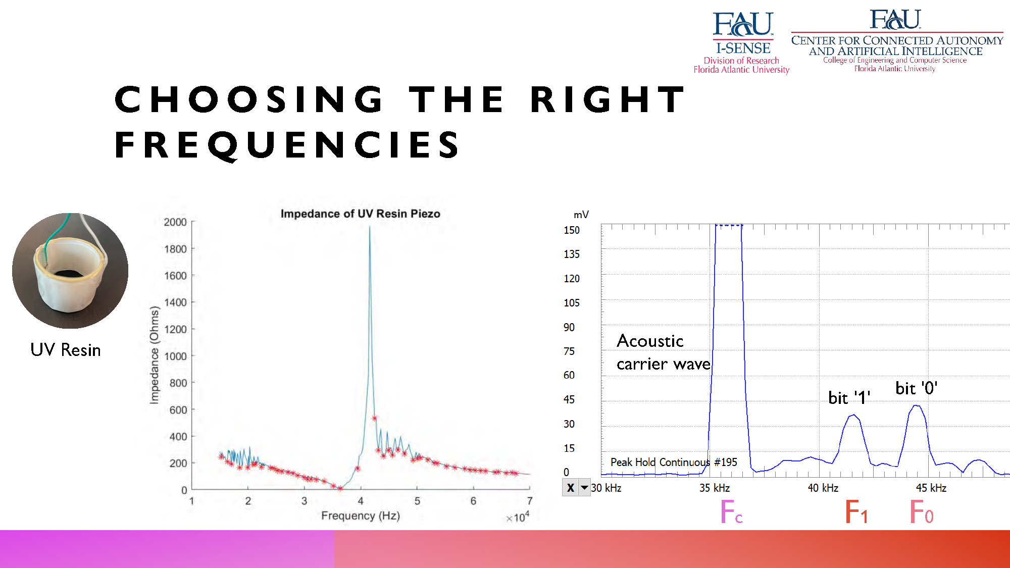
Choosing the Right Frequencies

On the left side, there's a small picture of the "UV Resin" piezo and a graph labeled "Impedance of UV Resin Piezo." The y-axis is "Impedance (Ohms)" and the x-axis is "Frequency (Hz)." The graph shows a line with a significant peak around 40 kHz. On the right side, there is a graph with a y-axis in "mV" and an x-axis in "Frequency (Hz)," with labels for 30 kHz, 35 kHz, 40 kHz, and 45 kHz. The graph displays peaks labeled "$F_c$", "$F_1$", and "$F_0$". A text box points to the "$F_c$" peak and labels it "Acoustic carrier wave," while the "$F_1$" and "$F_0$" peaks are labeled "bit '1'" and "bit '0'," respectively.

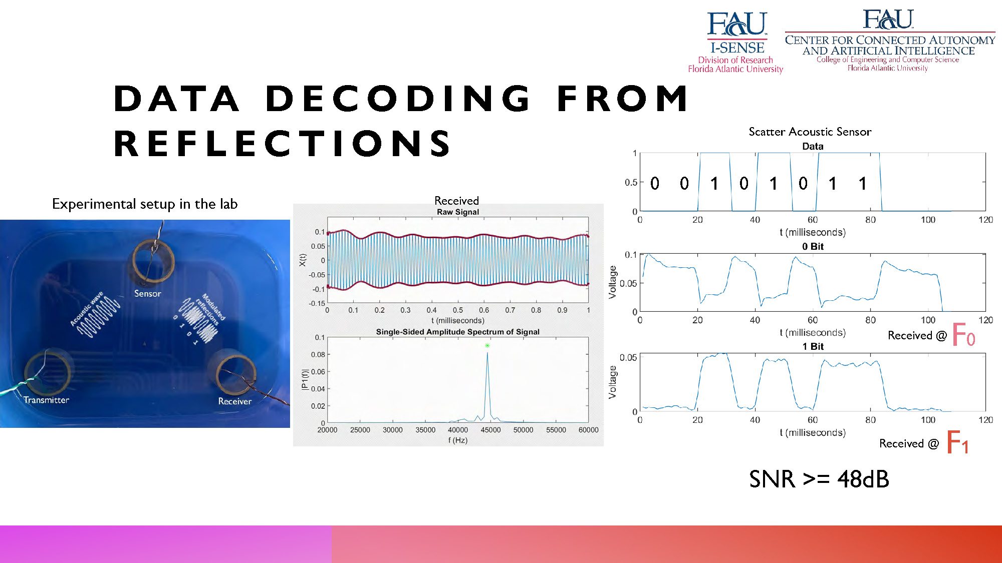
Data Decoding from Reflections

On the left side, a picture shows an "Experimental setup in the lab" inside a container with a "Transmitter," a "Sensor," and a "Receiver" labeled. The central section has two graphs: the top one is "Received Raw Signal" with the x-axis "t (milliseconds)" and the y-axis "X(t)," showing a wavy signal. The bottom graph is "Single-Sided Amplitude Spectrum of Signal," with the x-axis "f(Hz)" and the y-axis "P(f)," showing a single prominent peak. On the right, three graphs are stacked. The top graph is labeled "Scatter Acoustic Sensor Data" with the x-axis "t (milliseconds)" and y-axis "Data," showing a sequence of 0s and 1s. The middle and bottom graphs are labeled "0 Bit" and "1 Bit" respectively, with the x-axis "t (milliseconds)" and the y-axis "Voltage." The middle graph is also labeled "Received @ $F_0$" and the bottom graph is "Received @ $F_1$." The text "SNR >= 48dB" is at the bottom right.

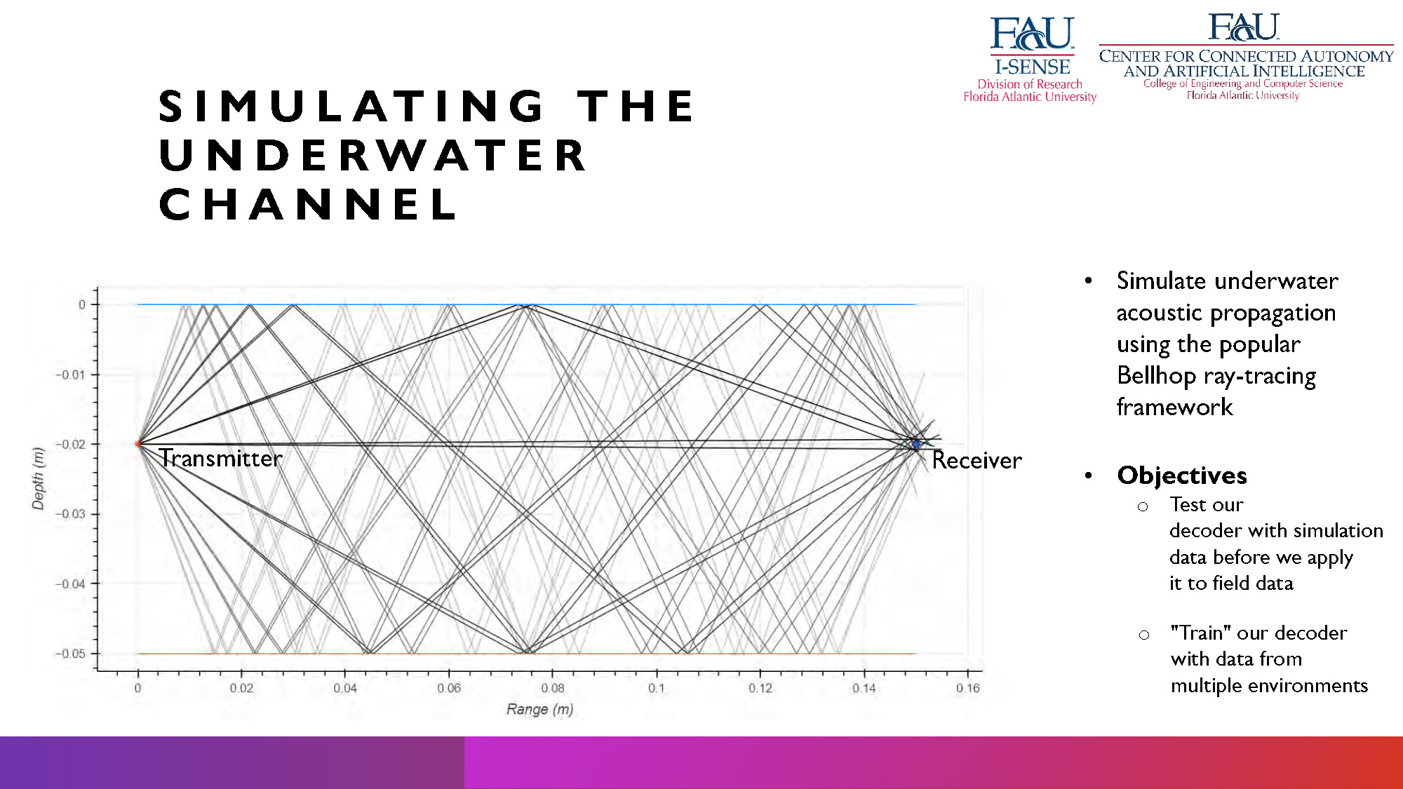
Simulating the Underwater Channel

Simulate underwater acoustic propagation using the popular Bellhop ray-tracing framework.

Objectives:

• Test the decoder with simulation data before applying it to field data
• "Train" the decoder with data from multiple environments

The visual is a graph with "Depth (m)" on the y-axis and "Range (m)" on the x-axis. It shows a series of lines representing paths between a "Transmitter" and a "Receiver."

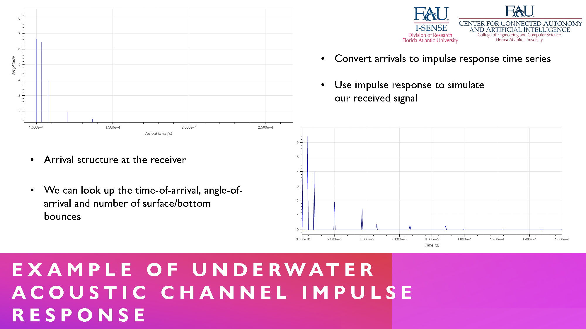
Example of Underwater Acoustic Channel Impulse Response

• Arrival structure at the receiver
• We can look up the time-of-arrival, angle-of-arrival and number of surface/bottom bounces
• Convert arrivals to impulse response time series
• Use impulse response to simulate the received signal

The top left features a graph with "Amplitude" on the y-axis and "Arrival time (s)" on the x-axis, showing several vertical lines. The bottom right displays a second graph with "Amplitude" on the y-axis and "Time (s)" on the x-axis, also showing a series of vertical lines.

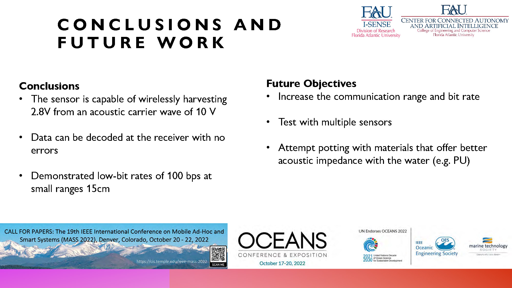
Conclusions and Future Work

Conclusions

• The sensor is capable of wirelessly harvesting 2.8V from an acoustic carrier wave of 10 V
• Data can be decoded at the receiver with no errors
• Demonstrated low-bit rates of 100 bps at small ranges 15cm

Future Objectives

• Increase the communication range and bit rate
• Test with multiple sensors
• Attempt potting with materials that offer better acoustic impedance with the water (e.g. PU)

End of Presentation

Click the right arrow to return to the beginning of the slide show.